Truncated normal distribution

In probability and statistics, the truncated normal distribution is the probability distribution derived from that of a normally distributed random variable by bounding the random variable from either below or above (or both). The truncated normal distribution has wide applications in statistics and econometrics. For example, it is used to model the probabilities of the binary outcomes in the probit model and to model censored data in the Tobit model.

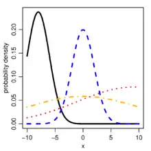
Probability density function Probability density function for the truncated normal distribution for different sets of parameters. In all cases, a = −10 and b = 10. For the black: μ = −8, σ = 2; blue: μ = 0, σ = 2; red: μ = 9, σ = 10; orange: μ = 0, σ = 10.
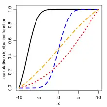
Cumulative distribution function Cumulative distribution function for the truncated normal distribution for different sets of parameters. In all cases, a = −10 and b = 10. For the black: μ = −8, σ = 2; blue: μ = 0, σ = 2; red: μ = 9, σ = 10; orange: μ = 0, σ = 10.
Notation	${\displaystyle \xi ={\frac {x-\mu }{\sigma }},\ \alpha ={\frac {a-\mu }{\sigma }},\ \beta ={\frac {b-\mu }{\sigma }}}$ ${\displaystyle Z=\Phi (\beta )-\Phi (\alpha )}$
Parameters	μ ∈ R σ^2 ≥ 0 (but see definition) a ∈ R — minimum value of x b ∈ R — maximum value of x (b > a)
Support	x ∈ [a,b]
PDF	${\displaystyle f(x;\mu ,\sigma ,a,b)={\frac {\phi (\xi )}{\sigma Z}}\,}$[1]
CDF	${\displaystyle F(x;\mu ,\sigma ,a,b)={\frac {\Phi (\xi )-\Phi (\alpha )}{Z}}}$
Mean	${\displaystyle \mu +{\frac {\phi (\alpha )-\phi (\beta )}{Z}}\sigma }$
Median	${\displaystyle \mu +\Phi ^{-1}\left({\frac {\Phi (\alpha )+\Phi (\beta )}{2}}\right)\sigma }$
Mode	${\displaystyle \left\{{\begin{array}{ll}a,&\mathrm {if} \ \mu <a\\\mu ,&\mathrm {if} \ a\leq \mu \leq b\\b,&\mathrm {if} \ \mu >b\end{array}}\right.}$
Variance	${\displaystyle \sigma ^{2}\left[1+{\frac {\alpha \phi (\alpha )-\beta \phi (\beta )}{Z}}-\left({\frac {\phi (\alpha )-\phi (\beta )}{Z}}\right)^{2}\right]}$
Entropy	${\displaystyle \ln({\sqrt {2\pi e}}\sigma Z)+{\frac {\alpha \phi (\alpha )-\beta \phi (\beta )}{2Z}}}$
MGF	${\displaystyle e^{\mu t+\sigma ^{2}t^{2}/2}\left[{\frac {\Phi (\beta -\sigma t)-\Phi (\alpha -\sigma t)}{\Phi (\beta )-\Phi (\alpha )}}\right]}$

Definitions

Suppose ${\displaystyle X}$ has a normal distribution with mean ${\displaystyle \mu }$ and variance ${\displaystyle \sigma ^{2}}$ and lies within the interval ${\displaystyle (a,b),{\text{with}}\;-\infty \leq a<b\leq \infty }$. Then ${\displaystyle X}$ conditional on ${\displaystyle a<X<b}$ has a truncated normal distribution.

Its probability density function, ${\displaystyle f}$, for ${\displaystyle a\leq x\leq b}$, is given by

${\displaystyle f(x;\mu ,\sigma ,a,b)={\frac {1}{\sigma }}\,{\frac {\phi ({\frac {x-\mu }{\sigma }})}{\Phi ({\frac {b-\mu }{\sigma }})-\Phi ({\frac {a-\mu }{\sigma }})}}}$

and by ${\displaystyle f=0}$ otherwise.

Here,

${\displaystyle \phi (\xi )={\frac {1}{\sqrt {2\pi }}}\exp \left(-{\frac {1}{2}}\xi ^{2}\right)}$

is the probability density function of the standard normal distribution and ${\displaystyle \Phi (\cdot )}$ is its cumulative distribution function

${\displaystyle \Phi (x)={\frac {1}{2}}\left(1+\operatorname {erf} (x/{\sqrt {2}})\right).}$

By definition, if ${\displaystyle b=\infty }$, then ${\displaystyle \Phi \left({\tfrac {b-\mu }{\sigma }}\right)=1}$, and similarly, if ${\displaystyle a=-\infty }$, then ${\displaystyle \Phi \left({\tfrac {a-\mu }{\sigma }}\right)=0}$.

The above formulae show that when ${\displaystyle -\infty <a<b<+\infty }$ the scale parameter ${\displaystyle \sigma ^{2}}$ of the truncated normal distribution is allowed to assume negative values. The parameter ${\displaystyle \sigma }$ is in this case imaginary, but the function ${\displaystyle f}$ is nevertheless real, positive, and normalizable. The scale parameter ${\displaystyle \sigma ^{2}}$ of the canonical normal distribution must be positive because the distribution would not be normalizable otherwise. The doubly truncated normal distribution, on the other hand, can in principle have a negative scale parameter (which is different from the variance, see summary formulae), because no such integrability problems arise on a bounded domain. In this case the distribution cannot be interpreted as a canonical normal conditional on ${\displaystyle a<X<b}$, of course, but can still be interpreted as a maximum-entropy distribution with first and second moments as constraints, and has an additional peculiar feature: it presents two local maxima instead of one, located at ${\displaystyle x=a}$ and ${\displaystyle x=b}$.

Properties

The truncated normal is the maximum entropy probability distribution for a fixed mean and variance, with the random variate X constrained to be in the interval [a,b].

Moments

If the random variable has been truncated only from below, some probability mass has been shifted to higher values, giving a first-order stochastically dominating distribution and hence increasing the mean to a value higher than the mean ${\displaystyle \mu }$ of the original normal distribution. Likewise, if the random variable has been truncated only from above, the truncated distribution has a mean less than ${\displaystyle \mu .}$

Regardless of whether the random variable is bounded above, below, or both, the truncation is a mean-preserving contraction combined with a mean-changing rigid shift, and hence the variance of the truncated distribution is less than the variance ${\displaystyle \sigma ^{2}}$ of the original normal distribution.

Two sided truncation[2]

Let ${\displaystyle \alpha =(a-\mu )/\sigma }$ and ${\displaystyle \beta =(b-\mu )/\sigma }$. Then:

${\displaystyle \operatorname {E} (X\mid a<X<b)=\mu +\sigma {\frac {\phi (\alpha )-\phi (\beta )}{\Phi (\beta )-\Phi (\alpha )}}\!}$

and

${\displaystyle \operatorname {Var} (X\mid a<X<b)=\sigma ^{2}\left[1+{\frac {\alpha \phi (\alpha )-\beta \phi (\beta )}{\Phi (\beta )-\Phi (\alpha )}}-\left({\frac {\phi (\alpha )-\phi (\beta )}{\Phi (\beta )-\Phi (\alpha )}}\right)^{2}\right]\!}$

Care must be taken in the numerical evaluation of these formulas, which can result in catastrophic cancellation when the interval ${\displaystyle [a,b]}$ does not include ${\displaystyle \mu }$. There are better ways to rewrite them that avoid this issue.[3]

One sided truncation (of lower tail)[4]

In this case ${\displaystyle \;b=\infty ,\;\phi (\beta )=0,\;\Phi (\beta )=1,}$ then

${\displaystyle \operatorname {E} (X\mid X>a)=\mu +\sigma \phi (\alpha )/Z,\!}$

and

${\displaystyle \operatorname {Var} (X\mid X>a)=\sigma ^{2}[1+\alpha \phi (\alpha )/Z-(\phi (\alpha )/Z)^{2}],}$

where ${\displaystyle Z=1-\Phi (\alpha ).}$

One sided truncation (of upper tail)

In this case ${\displaystyle \;a=\alpha =-\infty ,\;\phi (\alpha )=0,\;\Phi (\alpha )=0,}$ then

${\displaystyle \operatorname {E} (X\mid X<b)=\mu -\sigma {\frac {\phi (\beta )}{\Phi (\beta )}}\!}$,

${\displaystyle \operatorname {Var} (X\mid X<b)=\sigma ^{2}\left[1-\beta {\frac {\phi (\beta )}{\Phi (\beta )}}-\left({\frac {\phi (\beta )}{\Phi (\beta )}}\right)^{2}\right].\!}$

Barr and Sherrill (1999) give a simpler expression for the variance of one sided truncations. Their formula is in terms of the chi-square CDF, which is implemented in standard software libraries. Bebu and Mathew (2009) provide formulas for (generalized) confidence intervals around the truncated moments.

A recursive formula

As for the non-truncated case, there is a recursive formula for the truncated moments.[5]

Multivariate

Computing the moments of a multivariate truncated normal is harder.

Computational methods

Generating values from the truncated normal distribution

A random variate x defined as ${\displaystyle x=\Phi ^{-1}(\Phi (\alpha )+U\cdot (\Phi (\beta )-\Phi (\alpha )))\sigma +\mu }$ with ${\displaystyle \Phi }$ the cumulative distribution function and ${\displaystyle \Phi ^{-1}}$ its inverse, ${\displaystyle U}$ a uniform random number on ${\displaystyle (0,1)}$, follows the distribution truncated to the range ${\displaystyle (a,b)}$. This is simply the inverse transform method for simulating random variables. Although one of the simplest, this method can either fail when sampling in the tail of the normal distribution,[6] or be much too slow.[7] Thus, in practice, one has to find alternative methods of simulation.

One such truncated normal generator (implemented in Matlab and in R (programming language) as trandn.R ) is based on an acceptance rejection idea due to Marsaglia.[8] Despite the slightly suboptimal acceptance rate of Marsaglia (1964) in comparison with Robert (1995), Marsaglia's method is typically faster,[7] because it does not require the costly numerical evaluation of the exponential function.

For more on simulating a draw from the truncated normal distribution, see Robert (1995), Lynch (2007) Section 8.1.3 (pages 200–206), Devroye (1986). The MSM package in R has a function, rtnorm, that calculates draws from a truncated normal. The truncnorm package in R also has functions to draw from a truncated normal.

Chopin (2011) proposed (arXiv) an algorithm inspired from the Ziggurat algorithm of Marsaglia and Tsang (1984, 2000), which is usually considered as the fastest Gaussian sampler, and is also very close to Ahrens’s algorithm (1995). Implementations can be found in C, C++, Matlab and Python.

Sampling from the multivariate truncated normal distribution is considerably more difficult.[9] Exact or perfect simulation is only feasible in the case of truncation of the normal distribution to a polytope region.[9] [10] In more general cases, Damien and Walker (2001) introduce a general methodology for sampling truncated densities within a Gibbs sampling framework. Their algorithm introduces one latent variable and, within a Gibbs sampling framework, it is more computationally efficient than the algorithm of Robert (1995).

See also

• Folded normal distribution
• Half-normal distribution
• Normal distribution
• Rectified Gaussian distribution
• Truncated distribution
• PERT distribution

Notes

1. "Lecture 4: Selection" (PDF). web.ist.utl.pt. Instituto Superior Técnico. November 11, 2002. p. 1. Retrieved 14 July 2015.
2. Johnson, N.L., Kotz, S., Balakrishnan, N. (1994) Continuous Univariate Distributions, Volume 1, Wiley. ISBN 0-471-58495-9 (Section 10.1)
3. Fernandez-de-Cossio-Diaz, Jorge (2017-12-06), TruncatedNormal.jl: Compute mean and variance of the univariate truncated normal distribution (works far from the peak), retrieved 2017-12-06
4. Greene, William H. (2003). Econometric Analysis (5th ed.). Prentice Hall. ISBN 978-0-13-066189-0.
5. Document by Eric Orjebin, "https://people.smp.uq.edu.au/YoniNazarathy/teaching_projects/studentWork/EricOrjebin_TruncatedNormalMoments.pdf"
6. Kroese, D. P.; Taimre, T.; Botev, Z. I. (2011). Handbook of Monte Carlo methods. John Wiley & Sons.
7. Botev, Z. I.; L'Ecuyer, P. (2017). "Simulation from the Normal Distribution Truncated to an Interval in the Tail". 10th EAI International Conference on Performance Evaluation Methodologies and Tools. 25th–28th Oct 2016 Taormina, Italy: ACM. pp. 23–29. doi:10.4108/eai.25-10-2016.2266879. ISBN 978-1-63190-141-6.CS1 maint: location (link)
8. Marsaglia, George (1964). "Generating a variable from the tail of the normal distribution". Technometrics. 6 (1): 101–102. doi:10.2307/1266749. JSTOR 1266749.
9. Botev, Z. I. (2016). "The normal law under linear restrictions: simulation and estimation via minimax tilting". Journal of the Royal Statistical Society, Series B. 79: 125–148. arXiv:1603.04166. doi:10.1111/rssb.12162. S2CID 88515228.
10. Botev, Zdravko & L'Ecuyer, Pierre (2018). "Chapter 8: Simulation from the Tail of the Univariate and Multivariate Normal Distribution". In Puliafito, Antonio (ed.). Systems Modeling: Methodologies and Tools. EAI/Springer Innovations in Communication and Computing. Springer, Cham. pp. 115–132. doi:10.1007/978-3-319-92378-9_8. ISBN 978-3-319-92377-2. S2CID 125554530.

References

• Greene, William H. (2003). Econometric Analysis (5th ed.). Prentice Hall. ISBN 978-0-13-066189-0.
• Norman L. Johnson and Samuel Kotz (1970). Continuous univariate distributions-1, chapter 13. John Wiley & Sons.
• Lynch, Scott (2007). Introduction to Applied Bayesian Statistics and Estimation for Social Scientists. New York: Springer. ISBN 978-1-4419-2434-6.
• Robert, Christian P. (1995). "Simulation of truncated normal variables". Statistics and Computing. 5 (2): 121–125. arXiv:0907.4010. doi:10.1007/BF00143942. S2CID 15943491.
• Barr, Donald R.; Sherrill, E.Todd (1999). "Mean and variance of truncated normal distributions". The American Statistician. 53 (4): 357–361. doi:10.1080/00031305.1999.10474490.
• Bebu, Ionut; Mathew, Thomas (2009). "Confidence intervals for limited moments and truncated moments in normal and lognormal models". Statistics and Probability Letters. 79 (3): 375–380. doi:10.1016/j.spl.2008.09.006.
• Damien, Paul; Walker, Stephen G. (2001). "Sampling truncated normal, beta, and gamma densities". Journal of Computational and Graphical Statistics. 10 (2): 206–215. doi:10.1198/10618600152627906. S2CID 123156320.
• Nicolas Chopin, "Fast simulation of truncated Gaussian distributions". Statistics and Computing 21(2): 275-288, 2011, doi:10.1007/s11222-009-9168-1
• Burkardt, John. "The Truncated Normal Distribution" (PDF). Department of Scientific Computing website. Florida State University. Retrieved 15 February 2018.