Real coordinate space

In mathematics, a real coordinate space of dimension n, written Rⁿ (/ɑːrˈɛn/ ar-EN) or ℝⁿ, is a coordinate space over the real numbers. This means that it is the set of the n-tuples of real numbers (sequences of n real numbers). With component-wise addition and scalar multiplication, it is a real vector space.

The Cartesian product structure of R² on Cartesian plane of ordered pairs (x, y). Blue lines denote coordinate axes, horizontal green lines are integer y, vertical cyan lines are integer x, brown-orange lines show half-integer x or y, magenta and its tint show multiples of one tenth (best seen under magnification)

Typically, the Cartesian coordinates of the elements of a Euclidean space form a real coordinate space. This explains the name of coordinate space and the fact that geometric terms are often used when working with coordinate spaces. For example, R² is a plane.

Coordinate spaces are widely used in geometry and physics, as their elements allow locating points in Euclidean spaces, and computing with them.

Definition and structures

For any natural number n, the set Rⁿ consists of all n-tuples of real numbers (R). It is called the "n-dimensional real space" or the "real n-space".

An element of Rⁿ is thus a n-tuple, and is written

${\displaystyle (x_{1},x_{2},\ldots ,x_{n})}$

where each x_i is a real number. So, in multivariable calculus, the domain of a function of several real variables and the codomain of a real vector valued function are subsets of Rⁿ for some n.

The real n-space has several further properties, notably:

• With componentwise addition and scalar multiplication, it is a real vector space. Every n-dimensional real vector space is isomorphic to it.
• With the dot product (sum of the term by term product of the components), it is an inner product space. Every n-dimensional real inner product space is isomorphic to it.
• As every inner product space, it is a topological space, and a topological vector space.
• It is a Euclidean space and a real affine space, and every Euclidean or affine space is isomorphic to it.
• It is an analytic manifold, and can be considered as the prototype of all manifolds, as, by definition, a manifold is, near each point, isomorphic to an open subset of Rⁿ.
• It is an algebraic variety, and every real algebraic variety is a subset of Rⁿ.

These properties and structures of Rⁿ make it fundamental in almost all areas of mathematics and their application domains, such as statistics, probability theory, and many parts of physics.

The domain of a function of several variables

Any function f(x₁, x₂, … , x_n) of n real variables can be considered as a function on Rⁿ (that is, with Rⁿ as its domain). The use of the real n-space, instead of several variables considered separately, can simplify notation and suggest reasonable definitions. Consider, for n = 2, a function composition of the following form:

${\displaystyle F(t)=f(g_{1}(t),g_{2}(t)),}$

where functions g₁ and g₂ are continuous. If

∀x₁ ∈ R : f(x₁, ·) is continuous (by x₂)

∀x₂ ∈ R : f(·, x₂) is continuous (by x₁)

then F is not necessarily continuous. Continuity is a stronger condition: the continuity of f in the natural R² topology (discussed below), also called multivariable continuity, which is sufficient for continuity of the composition F.

Vector space

The coordinate space Rⁿ forms an n-dimensional vector space over the field of real numbers with the addition of the structure of linearity, and is often still denoted Rⁿ. The operations on Rⁿ as a vector space are typically defined by

${\displaystyle \mathbf {x} +\mathbf {y} =(x_{1}+y_{1},x_{2}+y_{2},\ldots ,x_{n}+y_{n})}$

${\displaystyle \alpha \mathbf {x} =(\alpha x_{1},\alpha x_{2},\ldots ,\alpha x_{n}).}$

The zero vector is given by

${\displaystyle \mathbf {0} =(0,0,\ldots ,0)}$

and the additive inverse of the vector x is given by

${\displaystyle -\mathbf {x} =(-x_{1},-x_{2},\ldots ,-x_{n}).}$

This structure is important because any n-dimensional real vector space is isomorphic to the vector space Rⁿ.

Matrix notation

In standard matrix notation, each element of Rⁿ is typically written as a column vector

${\displaystyle \mathbf {x} ={\begin{bmatrix}x_{1}\\x_{2}\\\vdots \\x_{n}\end{bmatrix}}}$

and sometimes as a row vector:

${\displaystyle \mathbf {x} ={\begin{bmatrix}x_{1}&x_{2}&\dots &x_{n}\end{bmatrix}}.}$

The coordinate space Rⁿ may then be interpreted as the space of all n × 1 column vectors, or all 1 × n row vectors with the ordinary matrix operations of addition and scalar multiplication.

Linear transformations from Rⁿ to R^m may then be written as m × n matrices which act on the elements of Rⁿ via left multiplication (when the elements of Rⁿ are column vectors) and on elements of R^m via right multiplication (when they are row vectors). The formula for left multiplication, a special case of matrix multiplication, is:

${\displaystyle (A{\mathbf {x} })_{k}=\sum \limits _{l=1}^{n}A_{kl}x_{l}}$

Any linear transformation is a continuous function (see below). Also, a matrix defines an open map from Rⁿ to R^m if and only if the rank of the matrix equals to m.

Standard basis

The coordinate space Rⁿ comes with a standard basis:

${\displaystyle {\begin{aligned}\mathbf {e} _{1}&=(1,0,\ldots ,0)\\\mathbf {e} _{2}&=(0,1,\ldots ,0)\\&{}\ \vdots \\\mathbf {e} _{n}&=(0,0,\ldots ,1)\end{aligned}}}$

To see that this is a basis, note that an arbitrary vector in Rⁿ can be written uniquely in the form

${\displaystyle \mathbf {x} =\sum _{i=1}^{n}x_{i}\mathbf {e} _{i}.}$

Geometric properties and uses

Orientation

The fact that real numbers, unlike many other fields, constitute an ordered field yields an orientation structure on Rⁿ. Any full-rank linear map of Rⁿ to itself either preserves or reverses orientation of the space depending on the sign of the determinant of its matrix. If one permutes coordinates (or, in other words, elements of the basis), the resulting orientation will depend on the parity of the permutation.

Diffeomorphisms of Rⁿ or domains in it, by their virtue to avoid zero Jacobian, are also classified to orientation-preserving and orientation-reversing. It has important consequences for the theory of differential forms, whose applications include electrodynamics.

Another manifestation of this structure is that the point reflection in Rⁿ has different properties depending on evenness of n. For even n it preserves orientation, while for odd n it is reversed (see also improper rotation).

Affine space

Rⁿ understood as an affine space is the same space, where Rⁿ as a vector space acts by translations. Conversely, a vector has to be understood as a "difference between two points", usually illustrated by a directed line segment connecting two points. The distinction says that there is no canonical choice of where the origin should go in an affine n-space, because it can be translated anywhere.

Convexity

The n-simplex (see below) is the standard convex set, that maps to every polytope, and is the intersection of the standard (n + 1) affine hyperplane (standard affine space) and the standard (n + 1) orthant (standard cone).

In a real vector space, such as Rⁿ, one can define a convex cone, which contains all non-negative linear combinations of its vectors. Corresponding concept in an affine space is a convex set, which allows only convex combinations (non-negative linear combinations that sum to 1).

In the language of universal algebra, a vector space is an algebra over the universal vector space R^∞ of finite sequences of coefficients, corresponding to finite sums of vectors, while an affine space is an algebra over the universal affine hyperplane in this space (of finite sequences summing to 1), a cone is an algebra over the universal orthant (of finite sequences of nonnegative numbers), and a convex set is an algebra over the universal simplex (of finite sequences of nonnegative numbers summing to 1). This geometrizes the axioms in terms of "sums with (possible) restrictions on the coordinates".

Another concept from convex analysis is a convex function from Rⁿ to real numbers, which is defined through an inequality between its value on a convex combination of points and sum of values in those points with the same coefficients.

Euclidean space

The dot product

${\displaystyle \mathbf {x} \cdot \mathbf {y} =\sum _{i=1}^{n}x_{i}y_{i}=x_{1}y_{1}+x_{2}y_{2}+\cdots +x_{n}y_{n}}$

defines the norm |x| = √x ⋅ x on the vector space Rⁿ. If every vector has its Euclidean norm, then for any pair of points the distance

${\displaystyle d(\mathbf {x} ,\mathbf {y} )=\|\mathbf {x} -\mathbf {y} \|={\sqrt {\sum _{i=1}^{n}(x_{i}-y_{i})^{2}}}}$

is defined, providing a metric space structure on Rⁿ in addition to its affine structure.

As for vector space structure, the dot product and Euclidean distance usually are assumed to exist in Rⁿ without special explanations. However, the real n-space and a Euclidean n-space are distinct objects, strictly speaking. Any Euclidean n-space has a coordinate system where the dot product and Euclidean distance have the form shown above, called Cartesian. But there are many Cartesian coordinate systems on a Euclidean space.

Conversely, the above formula for the Euclidean metric defines the standard Euclidean structure on Rⁿ, but it is not the only possible one. Actually, any positive-definite quadratic form q defines its own "distance" √q(x − y), but it is not very different from the Euclidean one in the sense that

${\displaystyle \exists C_{1}>0,\ \exists C_{2}>0,\ \forall \mathbf {x} ,\mathbf {y} \in \mathbb {R} ^{n}:C_{1}d(\mathbf {x} ,\mathbf {y} )\leq {\sqrt {q(\mathbf {x} -\mathbf {y} )}}\leq C_{2}d(\mathbf {x} ,\mathbf {y} ).}$

Such a change of the metric preserves some of its properties, for example the property of being a complete metric space. This also implies that any full-rank linear transformation of Rⁿ, or its affine transformation, does not magnify distances more than by some fixed C₂, and does not make distances smaller than 1 ∕ C₁ times, a fixed finite number times smaller.

The aforementioned equivalence of metric functions remains valid if √q(x − y) is replaced with M(x − y), where M is any convex positive homogeneous function of degree 1, i.e. a vector norm (see Minkowski distance for useful examples). Because of this fact that any "natural" metric on Rⁿ is not especially different from the Euclidean metric, Rⁿ is not always distinguished from a Euclidean n-space even in professional mathematical works.

In algebraic and differential geometry

Although the definition of a manifold does not require that its model space should be Rⁿ, this choice is the most common, and almost exclusive one in differential geometry.

On the other hand, Whitney embedding theorems state that any real differentiable m-dimensional manifold can be embedded into R^2m.

Other appearances

Other structures considered on Rⁿ include the one of a pseudo-Euclidean space, symplectic structure (even n), and contact structure (odd n). All these structures, although can be defined in a coordinate-free manner, admit standard (and reasonably simple) forms in coordinates.

Rⁿ is also a real vector subspace of Cⁿ which is invariant to complex conjugation; see also complexification.

Polytopes in Rⁿ

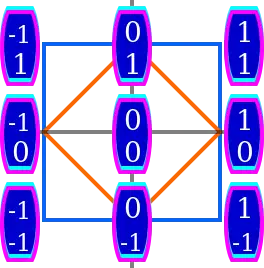
There are three families of polytopes which have simple representations in Rⁿ spaces, for any n, and can be used to visualize any affine coordinate system in a real n-space. Vertices of a hypercube have coordinates (x₁, x₂, … , x_n) where each x_k takes on one of only two values, typically 0 or 1. However, any two numbers can be chosen instead of 0 and 1, for example −1 and 1. An n-hypercube can be thought of as the Cartesian product of n identical intervals (such as the unit interval [0,1]) on the real line. As an n-dimensional subset it can be described with a system of 2n inequalities:

${\displaystyle \displaystyle {\begin{matrix}0\leq x_{1}\leq 1\\\vdots \\0\leq x_{n}\leq 1\end{matrix}}}$ (for [0,1])

${\displaystyle \displaystyle {\begin{matrix}|x_{1}|\leq 1\\\vdots \\|x_{n}|\leq 1\end{matrix}}}$ (for [−1,1])

Each vertex of the cross-polytope has, for some k, the x_k coordinate equal to ±1 and all other coordinates equal to 0 (such that it is the kth standard basis vector up to sign). This is a dual polytope of hypercube. As an n-dimensional subset it can be described with a single inequality which uses the absolute value operation:

${\displaystyle \sum \limits _{k=1}^{n}|x_{k}|\leq 1\,,}$

but this can be expressed with a system of 2ⁿ linear inequalities as well.

The third polytope with simply enumerable coordinates is the standard simplex, whose vertices are n standard basis vectors and the origin (0, 0, … , 0). As an n-dimensional subset it is described with a system of n + 1 linear inequalities:

${\displaystyle {\begin{matrix}0\leq x_{1}\\\vdots \\0\leq x_{n}\\\sum \limits _{k=1}^{n}x_{k}\leq 1\end{matrix}}}$

Replacement of all "≤" with "<" gives interiors of these polytopes.

Topological properties

The topological structure of Rⁿ (called standard topology, Euclidean topology, or usual topology) can be obtained not only from Cartesian product. It is also identical to the natural topology induced by Euclidean metric discussed above: a set is open in the Euclidean topology if and only if it contains an open ball around each of its points. Also, Rⁿ is a linear topological space (see continuity of linear maps above), and there is only one possible (non-trivial) topology compatible with its linear structure. As there are many open linear maps from Rⁿ to itself which are not isometries, there can be many Euclidean structures on Rⁿ which correspond to the same topology. Actually, it does not depend much even on the linear structure: there are many non-linear diffeomorphisms (and other homeomorphisms) of Rⁿ onto itself, or its parts such as a Euclidean open ball or the interior of a hypercube).

Rⁿ has the topological dimension n. An important result on the topology of Rⁿ, that is far from superficial, is Brouwer's invariance of domain. Any subset of Rⁿ (with its subspace topology) that is homeomorphic to another open subset of Rⁿ is itself open. An immediate consequence of this is that R^m is not homeomorphic to Rⁿ if m ≠ n – an intuitively "obvious" result which is nonetheless difficult to prove.

Despite the difference in topological dimension, and contrary to a naïve perception, it is possible to map a lesser-dimensional real space continuously and surjectively onto Rⁿ. A continuous (although not smooth) space-filling curve (an image of R¹) is possible.

Examples

Empty column vector, the only element of R^0

R^1

n ≤ 1

Cases of 0 ≤ n ≤ 1 do not offer anything new: R¹ is the real line, whereas R⁰ (the space containing the empty column vector) is a singleton, understood as a zero vector space. However, it is useful to include these as trivial cases of theories that describe different n.

n = 2

Both hypercube and cross-polytope in R² are squares, but coordinates of vertices are arranged differently

n = 3

Cube (the hypercube) and octahedron (the cross-polytope) of R³. Coordinates are not shown

n = 4

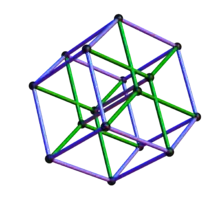
R⁴ can be imagined using the fact that 16 points (x₁, x₂, x₃, x₄), where each x_k is either 0 or 1, are vertices of a tesseract (pictured), the 4-hypercube (see above).

The first major use of R⁴ is a spacetime model: three spatial coordinates plus one temporal. This is usually associated with theory of relativity, although four dimensions were used for such models since Galilei. The choice of theory leads to different structure, though: in Galilean relativity the t coordinate is privileged, but in Einsteinian relativity it is not. Special relativity is set in Minkowski space. General relativity uses curved spaces, which may be thought of as R⁴ with a curved metric for most practical purposes. None of these structures provide a (positive-definite) metric on R⁴.

Euclidean R⁴ also attracts the attention of mathematicians, for example due to its relation to quaternions, a 4-dimensional real algebra themselves. See rotations in 4-dimensional Euclidean space for some information.

In differential geometry, n = 4 is the only case where Rⁿ admits a non-standard differential structure: see exotic R⁴.

Norms on Rⁿ

One could define many norms on the vector space Rⁿ. Some common examples are

• the p-norm, defined by ${\displaystyle ||{\textbf {x}}||_{p}:={\sqrt[{p}]{\sum _{i=1}^{n}|x_{i}|^{p}}}}$ for all ${\displaystyle {\textbf {x}}\in }$ Rⁿ where ${\displaystyle p}$ is a positive integer. The case ${\displaystyle p=2}$ is very important, because it is exactly the Euclidean norm.
• the ${\displaystyle \infty }$-norm or maximum norm, defined by ${\displaystyle ||{\textbf {x}}||_{\infty }:=\max\{x_{1},\dots ,x_{n}\}}$ for all ${\displaystyle {\textbf {x}}\in }$ Rⁿ. This is the limit of all the p-norms: ${\displaystyle ||{\textbf {x}}||_{\infty }=\lim \limits _{p\to \infty }{\sqrt[{p}]{\sum _{i=1}^{n}|x_{i}|^{p}}}}$.

A really surprising and helpful result is that every norm defined on Rⁿ is equivalent. This means for two arbitrary norms ${\displaystyle ||\cdot ||}$ and ${\displaystyle ||\cdot ||^{\prime }}$ on Rⁿ you can always find positive real numbers ${\displaystyle \alpha ,\beta >0}$, such that

${\displaystyle \alpha \cdot ||{\textbf {x}}||\leq ||{\textbf {x}}||^{\prime }\leq \beta \cdot ||{\textbf {x}}||}$ for all ${\displaystyle {\textbf {x}}\in }$ Rⁿ.

This defines an equivalence relation on the set of all norms on Rⁿ. With this result you can check that a sequence of vectors in Rⁿ converges with ${\displaystyle ||\cdot ||}$ if and only if it converges with ${\displaystyle ||\cdot ||^{\prime }}$.

Here is a sketch of what a proof of this result may look like:

Because of the equivalence relation it is enough to show that every norm on Rⁿ is equivalent to the Euclidean norm ${\displaystyle ||\cdot ||_{2}}$. Let ${\displaystyle ||\cdot ||}$ be an arbitrary norm on Rⁿ. The proof is divided in two steps:

• We show that there exists a ${\displaystyle \beta >0}$, such that ${\displaystyle ||{\textbf {x}}||\leq \beta \cdot ||{\textbf {x}}||_{2}}$ for all ${\displaystyle {\textbf {x}}\in }$ Rⁿ. In this step you use the fact that every ${\displaystyle {\textbf {x}}=(x_{1},\dots ,x_{n})\in }$ Rⁿ can be represented as a linear combination of the standard basis: ${\displaystyle {\textbf {x}}=\sum _{i=1}^{n}e_{i}\cdot x_{i}}$. Then with the Cauchy–Schwarz inequality ${\displaystyle ||{\textbf {x}}||=\left|\left|\sum _{i=1}^{n}e_{i}\cdot x_{i}\right|\right|\leq \sum _{i=1}^{n}||e_{i}||\cdot |x_{i}|\leq {\sqrt {\sum _{i=1}^{n}||e_{i}||^{2}}}\cdot {\sqrt {\sum _{i=1}^{n}|x_{i}|^{2}}}=\beta \cdot ||{\textbf {x}}||_{2}}$, where ${\displaystyle \beta$ :={\sqrt {\sum _{i=1}^{n}||e_{i}||^{2}}}} .
• Now we have to find an ${\displaystyle \alpha >0}$, such that ${\displaystyle \alpha \cdot ||{\textbf {x}}||_{2}\leq ||{\textbf {x}}||}$ for all ${\displaystyle {\textbf {x}}\in }$ Rⁿ. Assume there is no such ${\displaystyle \alpha }$. Then there exists for every ${\displaystyle k\in \mathbb {N} }$ a ${\displaystyle {\textbf {x}}_{k}\in }$ Rⁿ, such that ${\displaystyle ||{\textbf {x}}_{k}||_{2}>k\cdot ||{\textbf {x}}_{k}||}$. Define a second sequence ${\displaystyle ({\tilde {\textbf {x}}}_{k})_{k\in \mathbb {N} }}$ by ${\displaystyle {\tilde {\textbf {x}}}_{k}:={\frac {{\textbf {x}}_{k}}{||{\textbf {x}}_{k}||_{2}}}}$. This sequence is bounded because ${\displaystyle ||{\tilde {\textbf {x}}}_{k}||_{2}=1}$. So because of the Bolzano–Weierstrass theorem there exists a convergent subsequence ${\displaystyle ({\tilde {\textbf {x}}}_{k_{j}})_{j\in \mathbb {N} }}$ with limit ${\displaystyle {\textbf {a}}\in }$ Rⁿ. Now we show that ${\displaystyle ||{\textbf {a}}||_{2}=1}$ but ${\displaystyle {\textbf {a}}={\textbf {0}}}$, which is a contradiction. It is ${\displaystyle ||{\textbf {a}}||\leq ||{\textbf {a}}-{\tilde {\textbf {x}}}_{k_{j}}||+||{\tilde {\textbf {x}}}_{k_{j}}||\leq \beta \cdot ||{\textbf {a}}-{\tilde {\textbf {x}}}_{k_{j}}||_{2}+{\frac {||{\textbf {x}}_{k_{j}}||}{||{\textbf {x}}_{k_{j}}||_{2}}}\ {\overset {j\to \infty }{\to }}\ 0}$, because ${\displaystyle ||{\textbf {a}}-{\tilde {\textbf {x}}}_{k_{j}}||\to 0}$ and ${\displaystyle 0\leq {\frac {||{\textbf {x}}_{k_{j}}||}{||{\textbf {x}}_{k_{j}}||_{2}}}<{\frac {1}{k_{j}}}}$, so ${\displaystyle {\frac {||{\textbf {x}}_{k_{j}}||}{||{\textbf {x}}_{k_{j}}||_{2}}}\to 0}$. This implies ${\displaystyle ||{\textbf {a}}||=0}$, so ${\displaystyle {\textbf {a}}={\textbf {0}}}$. On the other hand ${\displaystyle ||{\textbf {a}}||_{2}=1}$, because ${\displaystyle ||{\textbf {a}}||_{2}=||\lim \limits _{j\to \infty }{\tilde {\textbf {x}}}_{k_{j}}||_{2}=\lim \limits _{j\to \infty }||{\tilde {\textbf {x}}}_{k_{j}}||_{2}=1}$. This can not ever be true, so the assumption was false and there exists such a ${\displaystyle \alpha >0}$.

See also

• Exponential object, for theoretical explanation of the superscript notation
• Real projective space

Footnotes

References

• Kelley, John L. (1975). General Topology. Springer-Verlag. ISBN 0-387-90125-6.
• Munkres, James (1999). Topology. Prentice-Hall. ISBN 0-13-181629-2.