Otsu's method
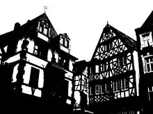
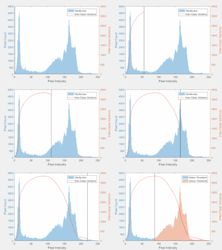
In computer vision and image processing, Otsu's method, named after Nobuyuki Otsu (大津展之, Ōtsu Nobuyuki), is used to perform automatic image thresholding.[1] In the simplest form, the algorithm returns a single intensity threshold that separate pixels into two classes, foreground and background. This threshold is determined by minimizing intra-class intensity variance, or equivalently, by maximizing inter-class variance.[2] Otsu's method is a one-dimensional discrete analog of Fisher's Discriminant Analysis, is related to Jenks optimization method, and is equivalent to a globally optimal k-means[3] performed on the intensity histogram. The extension to multi-level thresholding was described in the original paper,[2] and computationally efficient implementations have since been proposed.[4][5]


Otsu's method

The algorithm exhaustively searches for the threshold that minimizes the intra-class variance, defined as a weighted sum of variances of the two classes:
Weights and are the probabilities of the two classes separated by a threshold ,and and are variances of these two classes.
The class probability is computed from the bins of the histogram:
For 2 classes, minimizing the intra-class variance is equivalent to maximizing inter-class variance:[2]
which is expressed in terms of class probabilities and class means , where the class means , and are:
The following relations can be easily verified:
The class probabilities and class means can be computed iteratively. This idea yields an effective algorithm.
Algorithm
- Compute histogram and probabilities of each intensity level
- Set up initial and
- Step through all possible thresholds maximum intensity
- Update and
- Compute
- Desired threshold corresponds to the maximum
MATLAB or Octave implementation
histogramCounts is a 256-element histogram of a grayscale image different gray-levels (typical for 8-bit images). level is the threshold for the image (double).
function level = otsu(histogramCounts)
total = sum(histogramCounts); % total number of pixels in the image
%% OTSU automatic thresholding
top = 256;
sumB = 0;
wB = 0;
maximum = 0.0;
sum1 = dot(0:top-1, histogramCounts);
for ii = 1:top
    wF = total - wB;
    if wB > 0 && wF > 0
        mF = (sum1 - sumB) / wF;
        val = wB * wF * ((sumB / wB) - mF) * ((sumB / wB) - mF);
        if ( val >= maximum )
            level = ii;
            maximum = val;
        end
    end
    wB = wB + histogramCounts(ii);
    sumB = sumB + (ii-1) * histogramCounts(ii);
end
end
Matlab has built-in functions graythresh() and multithresh() in the Image Processing Toolbox which are implemented with Otsu's method and Multi Otsu's method, respectively.
Limitations
Otsu's method exhibits the relatively good performance if the histogram can be assumed to have bimodal distribution and assumed to possess a deep and sharp valley between two peaks. But if the object area is small compared with the background area, the histogram no longer exhibits bimodality.[6] And if the variances of the object and the background intensities are large compared to the mean difference, or the image is severely corrupted by additive noise, the sharp valley of the gray level histogram is degraded. Then the possibly incorrect threshold determined by Otsu's method results in the segmentation error. (Here we define the object size to be the ratio of the object area to the entire image area and the mean difference to be the difference of the average intensities of the object and the background)
Empirical results show that the performance of global thresholding techniques used for object segmentation (including Otsu's method) are limited by small object size, the small mean difference between foreground and background pixels, large variances of the pixels that belong to the object and those that belong to the background, the large amount of noise, etc.[7]
Improvements
Various extensions have been developed to address limitations of Otsu's method. One popular extension is the two-dimensional Otsu's method, which performs better for the object segmentation task in noisy images. Here, the intensity value of a given pixel is compared with the average intensity of its immediate neighborhood to improve segmentation results.[8]
At each pixel, the average gray-level value of the neighborhood is calculated. Let the gray level of the given pixel be divided into discrete values and the average gray level is also divided into the same values. Then a pair is formed: the pixel gray level and the average of the neighborhood . Each pair belongs to one of the possible 2-dimensional bins. The total number of occurrences (frequency), , of a pair , divided by the total number of pixels in the image , defines the joint probability mass function in a 2-dimensional histogram:
And the 2-dimensional Otsu's method is developed based on the 2-dimensional histogram as follows.
The probabilities of two classes can be denoted as:
The intensity mean value vectors of two classes and total mean vector can be expressed as follows:
In most cases the probability off-diagonal will be negligible, so it is easy to verify:
The inter-class discrete matrix is defined as
The trace of the discrete matrix can be expressed as
where
Similar to one-dimensional Otsu's method, the optimal threshold is obtained by maximizing .
Algorithm
The and is obtained iteratively which is similar with one-dimensional Otsu's method. The values of and are changed till we obtain the maximum of , that is
max,s,t = 0;
for ss: 0 to L-1 do
    for tt: 0 to L-1 do
        evaluate tr(S_b);
        if tr(S_b) > max
            max = tr(S,b);
            s = ss;
            t = tt;
        end if
    end for
end for
return s,t;
Notice that for evaluating , we can use a fast recursive dynamic programming algorithm to improve time performance.[9] However, even with the dynamic programming approach, 2d Otsu's method still has large time complexity. Therefore, much research has been done to reduce the computation cost.[10]
If summed area tables are used to build the 3 tables, sum over , sum over , and sum over , then the runtime complexity is the maximum of (O(N_pixels), O(N_bins*N_bins)). Note that if only coarse resolution is needed in terms of threshold, N_bins can be reduced.
Matlab implementation
function inputs and output:
hists is a 2D-histogram of grayscale value and neighborhood average grayscale value pair.
total is the number of pairs in the given image.it is determined by the number of the bins of 2D-histogram at each direction.
threshold is the threshold obtained.
function threshold = otsu_2D(hists, total)
maximum = 0.0;
threshold = 0;
helperVec = 0:255;
mu_t0 = sum(sum(repmat(helperVec',1,256).*hists));
mu_t1 = sum(sum(repmat(helperVec,256,1).*hists));
p_0 = zeros(256);
mu_i = p_0;
mu_j = p_0;
for ii = 1:256
    for jj = 1:256
        if jj == 1
            if ii == 1
                p_0(1,1) = hists(1,1);
            else
                p_0(ii,1) = p_0(ii-1,1) + hists(ii,1);
                mu_i(ii,1) = mu_i(ii-1,1)+(ii-1)*hists(ii,1);
                mu_j(ii,1) = mu_j(ii-1,1);
            end
        else
            p_0(ii,jj) = p_0(ii,jj-1)+p_0(ii-1,jj)-p_0(ii-1,jj-1)+hists(ii,jj);
            mu_i(ii,jj) = mu_i(ii,jj-1)+mu_i(ii-1,jj)-mu_i(ii-1,jj-1)+(ii-1)*hists(ii,jj);
            mu_j(ii,jj) = mu_j(ii,jj-1)+mu_j(ii-1,jj)-mu_j(ii-1,jj-1)+(jj-1)*hists(ii,jj);
        end

        if (p_0(ii,jj) == 0)
            continue;
        end
        if (p_0(ii,jj) == total)
            break;
        end
        tr = ((mu_i(ii,jj)-p_0(ii,jj)*mu_t0)^2 + (mu_j(ii,jj)-p_0(ii,jj)*mu_t1)^2)/(p_0(ii,jj)*(1-p_0(ii,jj)));

        if ( tr >= maximum )
            threshold = ii;
            maximum = tr;
        end
    end
end
end
References
- M. Sezgin & B. Sankur (2004). "Survey over image thresholding techniques and quantitative performance evaluation". Journal of Electronic Imaging. 13 (1): 146–165. doi:10.1117/1.1631315.
- Nobuyuki Otsu (1979). "A threshold selection method from gray-level histograms". IEEE Trans. Sys. Man. Cyber. 9 (1): 62–66. doi:10.1109/TSMC.1979.4310076.
- Liu, Dongju (2009). "Otsu method and K-means". Ninth International Conference on Hybrid Intelligent Systems IEEE. 1: 344–349.
- Liao, Ping-Sung (2001). "A fast algorithm for multilevel thresholding" (PDF). J. Inf. Sci. Eng. 17 (5): 713–727.
- Huang, Deng-Yuan (2009). "Optimal multi-level thresholding using a two-stage Otsu optimization approach". Pattern Recognition Letters. 30 (3): 275–284. doi:10.1016/j.patrec.2008.10.003.
- Kittler, Josef & Illingworth, John (1985). "On threshold selection using clustering criteria". IEEE Transactions on Systems, Man and Cybernetics. SMC-15 (5): 652–655. doi:10.1109/tsmc.1985.6313443.
- Lee, Sang Uk and Chung, Seok Yoon and Park, Rae Hong (1990). "A comparative performance study of several global thresholding techniques for segmentation". Computer Vision, Graphics, and Image Processing. 52 (2): 171–190. doi:10.1016/0734-189x(90)90053-x.CS1 maint: multiple names: authors list (link)
- Jianzhuang, Liu and Wenqing, Li and Yupeng, Tian (1991). "Automatic thresholding of gray-level pictures using two-dimension Otsu method". Circuits and Systems, 1991. Conference Proceedings, China., 1991 International Conference on: 325–327.CS1 maint: multiple names: authors list (link)
- Zhang, Jun & Hu, Jinglu (2008). "Image segmentation based on 2D Otsu method with histogram analysis". Computer Science and Software Engineering, 2008 International Conference on. 6: 105–108. doi:10.1109/CSSE.2008.206. ISBN 978-0-7695-3336-0.
- Zhu, Ningbo and Wang, Gang and Yang, Gaobo and Dai, Weiming (2009). "A fast 2d otsu thresholding algorithm based on improved histogram". Pattern Recognition, 2009. CCPR 2009. Chinese Conference on: 1–5.CS1 maint: multiple names: authors list (link)
External links
- Implementation of Otsu's thresholding method as GIMP-plugin using Script-Fu (a Scheme-based language)
- Lecture notes on thresholding – covers the Otsu method
- A plugin for ImageJ using Otsu's method to do the threshold
- A full explanation of Otsu's method with a working example and Java implementation
- Implementation of Otsu's method in ITK
- Otsu Thresholding in C# – a straightforward C# implementation with explanation
- Otsu's method using MATLAB
- Otsu Thresholding with scikit-image in Python