Semblance analysis
Semblance analysis is a process used in the refinement and study of seismic data. The use of this technique along with other methods makes it possible to greatly increase the resolution of the data despite the presence of background noise. The new data received following the semblance analysis is usually easier to interpret when trying to deduce the underground structure of an area. Weighted semblance can be used for increasing the resolution of traditional semblance or make traditional semblance capable of analyzing more complicated seismic data.[1][2][3]
History
Semblance analysis is a technique that first began to be developed and used in the late 1960s. Prior to the discovery of this method, identifying the main reflections produced by the many layers under the ground was fairly difficult. The primary reflections of these layers were often obscured by the background noise as well as noise from the many secondary reflections that are produced. The use of semblance analysis allows for the removal of the extra noise and leaves only the primary reflection.
Process


Semblance analysis allows for the refinement of seismic data. This is done by developing a velocity spectra[4] display to determine the velocity through different layers at depth.[5] The easiest way to accomplish this is by recording the normal incidence path (NIP). The NIP is where you have the shot and the geophone in the same location and the path taken by the recorded sound waves is perpendicular to the boundaries between the layers.[6] This path represents the shortest amount of time that can be taken to reach a layer and return. With this information it becomes fairly easy to calculate the velocity of the waves as they travel through each layer by using the equation for the root mean square velocity starting with the top layer and working downward.
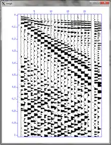
Once all of the velocities for the layers are known then it is possible to calculate the time needed for the wave to travel the distance down to the midpoint between each geophone and the shot point for each of the layers. As the geophones are farther away from the shot, the more the time taken for the wave to travel there increases, this forms a hyperbola in a graph of time vs. distance. The velocity data is used to correct the curves of the hyperbolas and create a flat line where all points are at an equal depth. The final step for the semblance analysis is to sum all of the data that has been corrected for velocity. This is done with the use of a computer filter to sum together all of the events that the traces share, then remove the ones they don't. The result is a single data set that has all of the primary peaks strongly displayed with most of the noise removed.[7]
Problems
While this technique can be very useful in the analysis there are several situations in which it will not work. Semblance analysis will not work properly when the offset from the shot is greater than the depth of the reflecting layers because the data no longer has a hyperbolic pattern. To correct this it is necessary to use more complex equations that model non-hyperbolic moveout.[8] Also in situations where there is large offset there can also be polarity reversals with moveout then the data will be heavily distorted. To make moveout analysis suitable for data with polarity reversals a method known as AK semblance developed. This method first worked only for 2D models but has since been further refined for 3D as well.[9]
Code of program
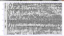
This code is for a program in Perl that allows for the determination of multiple moveout velocities for the correction of seismic data.
#!/bin/sh
set -x
# nmo_test.sh
# Nov. 8, 2012
# Program to test nmo's
# several constant velocity moveouts are tested
# starting at 60 m/s and ending at 1000 m/s
# STEP 1: Data is sorted by cdp and offset
# STEP 1A: Data is windowed
# STEP 2: DATA is moved out
# STEP 3: data is filtered
# STEP 4: data is gained
# STEP 5: data is displayed
# Juan M. Lorenzo
# set up working directories

SU_DIR='Directory'
this_file='input_file'
counter=0
vel_start=7500
vel_last=35000
vel_inc=5000
first_cmp=1
last_cmp=1
for ((vel=$vel_start; vel<=$vel_last; vel=$vel+$vel_inc))
do
	echo $vel
	susort <$SU_DIR/$this_file.su cdp offset	\
		|
	suwind key=cdp min=$first_cmp max=$last_cmp \
		|					\
	sunmo vnmo=$vel		\
		|					\
	sufilter f=0,3,400,600				\
		| 					\
	sugain agc=1 wagc=0.1				\
		|					\
	suximage   			\
							\
	xbox=$[$counter*200] ybox=0 wbox=200 hbox=600  	\
	title="$vel m/s" & 		\
	counter=$[$counter+1]
done
References
- Chen, Yangkang; Liu, Tingting; Chen, Xiaohong (July–August 2015). "Velocity analysis using similarity-weighted semblance". Geophysics. 80 (4): A75–A82. doi:10.1190/geo2014-0618.1.
- Gan, Shuwei; Wang, Shoudong; Chen, Yangkang; Qu, Shan; Zu, Shaohuan (2016). "Velocity analysis of simultaneous-source data using high-resolution semblance—coping with the strong noise". Geophysical Journal International. 204 (2): 768–779. doi:10.1093/gji/ggv484.
- Ebrahimi, Saleh; Kahoo, Amin; Chen, Yangkang; Porsani, Milton (March–April 2017). "A high-resolution weighted AB semblance for dealing with amplitude-variation-with-offset phenomenon". Geophysics. 82 (2): V85–V93. doi:10.1190/geo2016-0047.1.
- "Velocity Spectra". Stanford Exploration Project. Stanford University. 2000.
- M. TURHAN TANER; FULTON KOEHLERS; Society of Exploration Geophysicists (December 1969). "VELOCITY SPECTRA-DIGITAL COMPUTER DERIVATION AND APPLICATIONS OF VELOCITY FUNCTIONS" (PDF). GEOPHYSICS. p. 859.
- Schlumberger Limited (2020). "Oilfield Glossary: Normal Incidence".
- Taner, Turhan; Fulton Koehler (December 1969). "Velocity Spectra-Digital Computer Derivation and Application of Velocity Functions". Geophysics. 34 (6): 859–881. doi:10.1190/1.1440058.
- Sergey Fomel; Alexey Stovas. "Generalized nonhyperbolic moveout approximation". Geophysics. Society of Exploration Geophysicists. eISSN 1942-2156. ISSN 0016-8033 – via SEG Library.
- Yan, Jia; Ilya Tsvankin (March–April 2008). "AVO-sensitive semblance analysis for wide-azimuth data". Geophysics. 73 (2): U1–U11. doi:10.1190/1.2834115.